Encoded Walker, Part 1: From Random Walks to Radial Forms

The encoded walker project began with a simple question: what happens when you take the familiar random walk algorithm and bend it into a circle?

The Random Walk Foundation

A random walk is one of the most fundamental concepts in generative art and computational mathematics. At each step, an agent moves in a direction determined by some random or pseudo-random process. The beauty lies in the emergent paths that arise from accumulated small decisions.

In a traditional 2D random walk, each step might move left, right, up, or down with equal probability. The resulting path wanders through space, creating meandering trails that mirror natural phenomena like Brownian motion or the path of a foraging animal.

But truly random motion can be chaotic. What if we wanted something that felt organic without being erratic?

Noise Instead of Randomness

The key insight was to replace pure randomness with coherent noise. Perlin noise, developed by Ken Perlin for the original Tron film, provides smooth, continuous variation that changes gradually across space. Unlike random values that jump unpredictably, noise flows.

For each point in our walker, we sample the noise field at its current position:

nx = x + map(noise(x * busyness, y * busyness, time), 0, 1, -severity, severity)
ny = y + map(noise(y * busyness, x * busyness, time), 0, 1, -severity, severity)

The busyness parameter controls how quickly the noise varies spatially. Lower values create smooth, sweeping curves. Higher values create more turbulent, detailed displacement. The severity parameter scales the maximum displacement at each step.

By sampling 3D noise with a time parameter that increments with each generation step, we ensure that successive iterations produce related but distinct displacements. The curves evolve rather than jump.

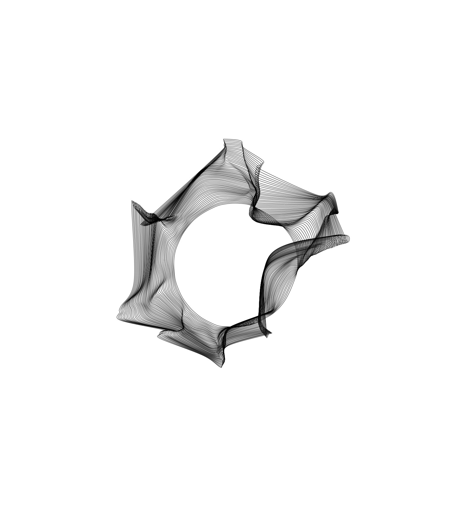
The Radial Arrangement

Here's where the encoding begins. Rather than starting from a single point or a line, we arrange our initial points in a circle:

for (int i = 0; i < numStartingPoints; i++) {
    float angle = TWO_PI * i / numStartingPoints;
    float x = centerX + radius * cos(angle);
    float y = centerY + radius * sin(angle);
    points.add(new PVector(x, y));
}

Each point occupies a position from 0 to 2π radians around the center. This angular distribution becomes significant later when we consider how information might be encoded in these forms.

Generational Iteration

With the initial arrangement established, we iterate. Each generation:

1. Displaces every point according to noise at its current position
2. Optionally pushes points outward with radial spacing
3. Connects the displaced points with Catmull-Rom splines

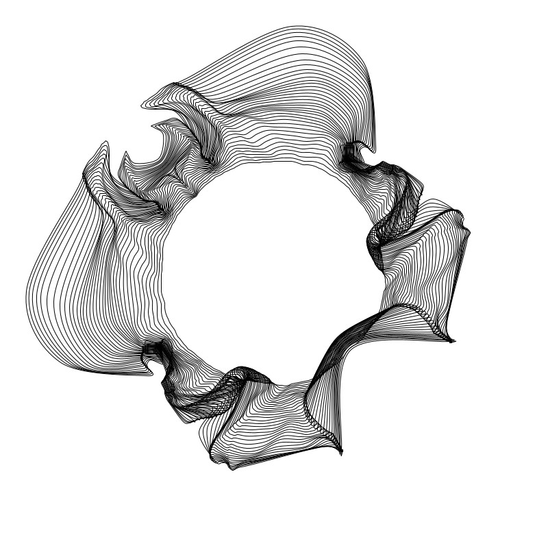
The radial spacing creates a layered effect. Early iterations stay close to the original circle while later iterations expand outward, preserving the visual history of the walk.

float offset = spacing * stepIndex;
nx = nx + (dx / dist) * offset;
ny = ny + (dy / dist) * offset;

Catmull-Rom Curves

Rather than connecting points with straight lines, we use Catmull-Rom splines. These interpolating splines pass through each control point while maintaining smooth continuity. The curve between any two points is influenced by the points before and after, creating naturalistic transitions.

Processing's curveVertex() function implements this automatically. To close the loop smoothly, we need to repeat the first few points at the end:

beginShape();
for (PVector pt : path) {
    curveVertex(pt.x, pt.y);
}
// Close smoothly
curveVertex(path.get(0).x, path.get(0).y);
curveVertex(path.get(1).x, path.get(1).y);
curveVertex(path.get(2).x, path.get(2).y);
endShape();

The Role of the Seed

Every generated form is reproducible. The seed value initializes both the random number generator and the noise function, ensuring that identical parameters produce identical output.

This reproducibility transforms the system from a mere generator into something more interesting: a deterministic mapping from parameters to forms. Given the same inputs, the same shape emerges. This property becomes crucial when we consider encoding and decoding information in Part 2.

Parameter Space

The final system exposes several parameters:

• Seed: The reproducibility key
• Starting points (3-200): Density of the radial distribution
• Steps (5-200): Number of generational iterations
• Spacing (0-10): Radial expansion between generations
• Severity (1-50): Maximum noise displacement
• Busyness (0.001-0.1): Noise spatial frequency
• Radius (50-400): Initial circle size

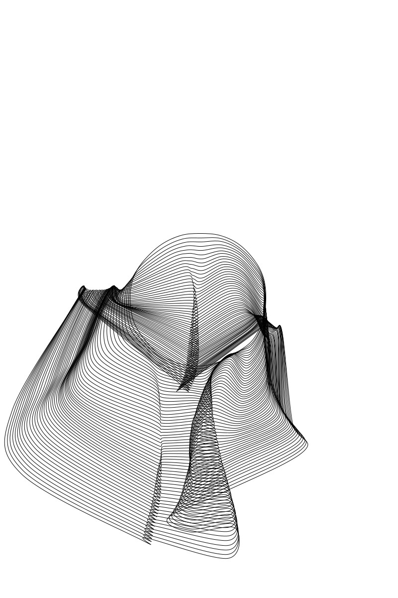
Each parameter combination defines a unique region in the space of possible forms. Low starting points with high steps create flowing ribbons. High starting points with low severity create dense, hair-like textures. The interactions are complex and often surprising.

Optional Directional Offset

A later addition to the system was directional offset. Rather than having curves purely expand radially, they can drift in a specified direction (down, right, or diagonally). This creates forms that seem to flow or fall, adding another dimension of expression.

Output Formats

The system exports in three formats:

• SVG: Vector format preserving the mathematical curves, with embedded metadata in XML
• PNG: Lossless raster at canvas resolution
• JPG: Compressed raster for web use

Each export includes a JSON sidecar containing all generation parameters, enabling full reproducibility and providing the foundation for potential decoding applications.

What's Next

In Part 2, we'll explore how these forms might encode information. Drawing from Morse code and other transmission schemes, we'll consider how the radial arrangement from 0 to 2π creates a natural alphabet, and how software might generate and decode messages hidden in curves.

The encoded walker isn't just a generative art system. It's a foundation for visual communication.